Data Download - First Modeling Round
Country level IMAGE 2.2 GDP data for Economic Optimism, Techno Garden & Elites (click to download Excel 390KB-file with GDP per capita and total GDP in 103 US$)
Economic Optimism:
GDP based on the GEO Market First scenario
Techno Garden :
GDP based on SRES B1 scenario
Elites :
GDP based on SRES A2 scenario
Downscaling IMAGE 2.2 data to country level (by Detlef van Vuuren)
CIESIN has downscaled both population and GDP data to the country level. The method for used population data seem to work well (see also memo Brian O’Neill). The method for income, however, seems to be inadequate. Here an alternative method is proposed.
Income
CIESIN has assumed that GDP of each country grows as fast as the regional aggregate, the latter based on the information in each of the markers. This methodology works adequately for a large number of countries, but produces very unlikely results for other countries. For Hong-Kong, for instance, assuming a growth rate on the basis of the East Asian average growth rate results in an income of 1.5 million US$ per capita in 2100 (current income is around 20,000 US$ per capita; income of the region is below 1,000 US$ and is projected to grow at rates above 5% per year in the next 30 years in A1). It can simply be concluded that the CIESIN downscaling method (although elegantly simple) is inadequate.
Assuming some form of partial convergence of countries within regions seems to be the logical solution to solve this. First of all, each of the SRES scenarios also assumes partial convergence in regional per capita income levels, so it seems logical to translate this rule also to lower levels. Second, high(er) income countries in low income regions can be expected to grow in a similar fashion as high(er) income countries in high-income regions. Assuming partial convergence of income within low-income regions may achieve this.
This means that a new method for downscaling needs to be developed. This method needs to comply with different criteria:
- It needs to produce reasonable results for growth rates for each of the countries (e.g. high income countries in low income regions not growing much faster than the average high income regional growth rates) by assuming some degree of convergence.
- The level of convergence needs to be made scenario dependent.
- The regional aggregation of the country data for GDP needs to be equal to the original IMAGE regions.
- The method needs to be relatively simple.
The method that provided that the best results at the moment is the following.
- We determine the hypothetical average growth rate for pcGDP (grC) of each country, assuming that it would converge to the income to the corresponding region in a certain year, e.g. 2200. This leads to complete converge of income in each region – however, as we will set this year outside the 2000-2100 time period, only partial convergence will be achieved in 2100. The regional income in the convergence year is estimated by extrapolating the regional growth trajectory of SRES.
- Next, we need to accommodate for the fact that in SRES almost all low income countries have significantly higher growth rates in the beginning of the century, while in contrast, most high income countries have more or less flat growth rates. Therefore, we first determine the relative growth rate of each region for different time periods compared to the average growth rate over the whole century RG (e.g. 2.0 in 2010 means that the growth in 2010 of that region is twice the average growth rate over the whole century for that region). Next, we assume that each country is coupled to a weighted average of two RGs, i.e. the RG of its own region and the average RG of the high income regions. The weighting is based on the ratio of the country’s income versus the average income of its region. Is the income of a country below, or close the region’s average – than also its growth is distributed as its own region. Is the income of a country much higher than the region’s average, than its growth is coupled to that of high income regions – and thus flat.
- In a last step, the GDP growth rates of all countries in a region needs to be adjusted in order to maintain strict parity between the sum of the country GDP and the regional growth rates of IMAGE. Obviously, the value of the correction is equal to the sum of the result of step 2 and the existing regional GDP IMAGE trajectories. Again, the actual correction is done weighted on the basis of the same ratio used in step 2 (thus exempting high income countries in low income regions), in order to avoid pulling up the growth rates of high income countries too much.
This method seems to result in reasonable results (maybe not perfect, but definitely better than the CIESIN method). Figure 1 shows the GDP per capita development of all 206 countries included in the downscaling for A1 and A2. For A1, the results are also shown in Table 1. Here, one can see that the CIESIN/Kassel first round method results in Hong-Kong already reaching income levels 8 times that of Canada in 2050. There is a group of about 10-20 (mostly small, exception Korea) countries with similar results. One could also note Argintina, over taking some of the rich countries in 2050 and going to a level almost 50% above the in 2100 – while leaving Brazil behind.
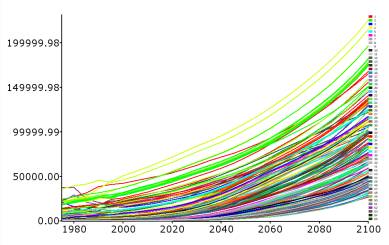
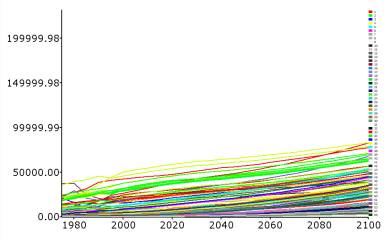
Figure 1: GDP per capita development of all 206 countries included in the downscaling for A1 and A2
| Current | method | CIESIN | method | |||||||||||
| 2000 | 2020 | 2050 | 2100 | 2000- | 2020- | 2050- | 2000 | 2020 | 2050 | 2100 | 2000- | 2020- | 2050- | |
| 2020 | 2050 | 2100 | 2020 | 2050 | 2100 | |||||||||
| Canada | 21836 | 30673 | 52843 | 136366 | 1.7% | 1.8% | 1.9% | 22195 | 30673 | 52843 | 136366 | 1.7% | 1.8% | 1.9% |
| United States | 32163 | 47154 | 74747 | 151291 | 1.9% | 1.5% | 1.4% | 31844 | 47154 | 74747 | 151291 | 1.9% | 1.5% | 1.4% |
| China | 799 | 4137 | 20667 | 75313 | 8.6% | 5.5% | 2.6% | 807 | 3049 | 13683 | 48144 | 6.9% | 5.1% | 2.5% |
| Hong Kong | 22582 | 34197 | 63161 | 122192 | 2.1% | 2.1% | 1.3% | 23280 | 87974 | 394843 | 1389267 | 6.9% | 5.1% | 2.5% |
| Germany | 32220 | 48249 | 79207 | 182526 | 2.0% | 1.7% | 1.7% | 32301 | 49643 | 84342 | 204852 | 2.2% | 1.8% | 1.8% |
| Brazil | 4708 | 10192 | 38211 | 110612 | 3.9% | 4.5% | 2.1% | 4560 | 9527 | 34921 | 103291 | 3.8% | 4.4% | 2.2% |
| Argentina | 8813 | 16028 | 45335 | 114683 | 3.0% | 3.5% | 1.9% | 8248 | 17229 | 63155 | 186801 | 3.8% | 4.4% | 2.2% |
Kassel has used the ‘CIESIN method’ in the previous round of MA analysis. I propose to use at this stage the new numbers as prepared on the basis of this note. In the future, it might be possible to refine the method further. back